Polynomial path planning in Frenet Frame

Frames of motion observation

• World Frame ${W}$: Inertial frame in 2D space. The most common coordinate is the rectangle coordinate (x-y).
  
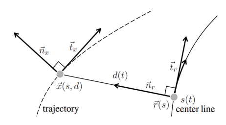
• Frenet Frame ${F}$: Frenet frame is a coordinate built on the curve. In 2D space, it is composed of four components: a point ($\vec{r}$) on the curve, tangential vector ($\vec{t_r}$), distance to the reference point ($d$),normal vector ($\vec{n_r}$).

Curve parameterization

In the rectangle coordinate, the curve can be expressed with $f(x,y)=0$. If we introduce an intermediate parameter $t$, the curve can be expressed with $x(t)$ and $y(t)$. Given the Frenet frame, we can choose arc length $s$ of the curve as the intermediate parameter. Givne that, any point in the 2D space can also be paramterized in the Frenet Frame after deciding the parameter $s$: $\vec{r(s)}$, d(s),$\vec{t_r(s)}$,$\vec{n_r(s)}$

Motion expression in Frenet Frame

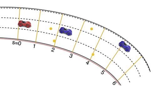
When there is an object moving in a 2D space, we can express the motion in the inertial frame with rectangle coordinates (x-y). The motion can be separated into two 1-D motions (along x and y) and combine them to the actual motion. Take velocity as an example, $\vec{v_x}+\vec{v_y}=\vec{v}$. Similarly, we can also express the motion in the Frenet Frame which is also inertial. As a result, the components to express the reference segment position on the curve is a function of time: $s(t)$ and the other components ($d$,$\vec{t_r}$,$\vec{n_r}$) are also the function of time. When we build a path planning to follow a global path, we can design its motion along $d$ and $s$ so that the planned path can be achieved to meet the requirements of the offset (d) to the path, as well as the velocity and acceleration on the path.

Transformation between rectangle coordinates (x-y) and Frenet Frame coordinates (s-d)

The motion transformation from x-y coordinate to Frenet Frame is essential, as we need to decide the start planning point in the Frenent Frame.

1. The position conversion:
   • $s,d → x,y$:
   • $\vec{x}=\vec{r}+d\vec{n_r}$, where $\vec{n_r}$ and $\vec{r}$ can be obtained from the parameterized curve.

• $x,y → s,d$: (the method is for discretized curve, the analytical expression is more accurate)
  • The nearest point to (x,y), $\vec{x}$ in 2D space is the reference point $\vec{r}(s)$, given $\vec{r}(s)$ we can also calculate the norm vector $\vec{n_r}$, so $d = (\vec{x}-\vec{r})^T\vec{n_r}$ ;
  • $s$ is the parameter arc segment;

1. The velocity conversion:
   • $v,\theta$ → $\dot{s},\dot{d}$:
   • $\theta_r$($\vec{t_r}$ to the x-axis) and $\kappa_r$ are obtained from the curve feature in the position conversion;
   • $\dot{d}=vsin(\theta - \theta_r)$
   • $\dot{s}=\frac{vcos(\theta - \theta_r)}{1-\kappa_rd}$ * $\dot{s},\dot{d}$ → $v,\theta$:
   • $v=\sqrt{\dot{s}^2(1-\kappa_rd)^2+\dot{d}^2}$
   • $\theta=arccos(\frac{\dot{s}(1-\kappa_rd)}{v}+\theta_r)$

For the actual robot motion, the acceleration observation normally sustain large amount of noise. Given enough time and small $\Delta v$, we can get a good planned path with the assumption that $\ddot{s}=0$. However, $\ddot{d}$ is not just relevant to the acceleration, but also the speed for the curve motion, so it cannot be ignored. The $\ddot{d}$ can be estimated with the equation:

where $\ddot{s}$ can be assumed to be zero for the small target v relative to the maximum allowed acceleration, so

where $d’’$ can be calculated from the below equation:

where $d’=(1-\kappa_rd)tan\Delta\theta$. \kappa_r’d can be calculated with the following equation:

where x’ and y’ are the parameterization of curve to the arc segment s.

Polynomial motion planning

Quntic path is a local path planner in real time with the objective of minimum jerk (time derivative of acceleration) along the path. The path planner will output the position, velocity and acceleration at each time stamp along the path. \(C=\frac{1}{2}\int_0^T L dt\) where L is the square of jerk:

Here x(t) and y(t) indicates the position components on x-y coordinate system. If x(t) and y(t) are sufficiently differential-able, the local optimal (extremum) points need to meet the following equations:

As we assume the path in time domain is continuous and derivative, the following polynomial equations for x(t) and y(t) can be used:

The parameters $a_i$ can be obtained given boundary conditions.